使用 R 中的 tidymodels 获取 catboost 模型的摘要形状图

Question

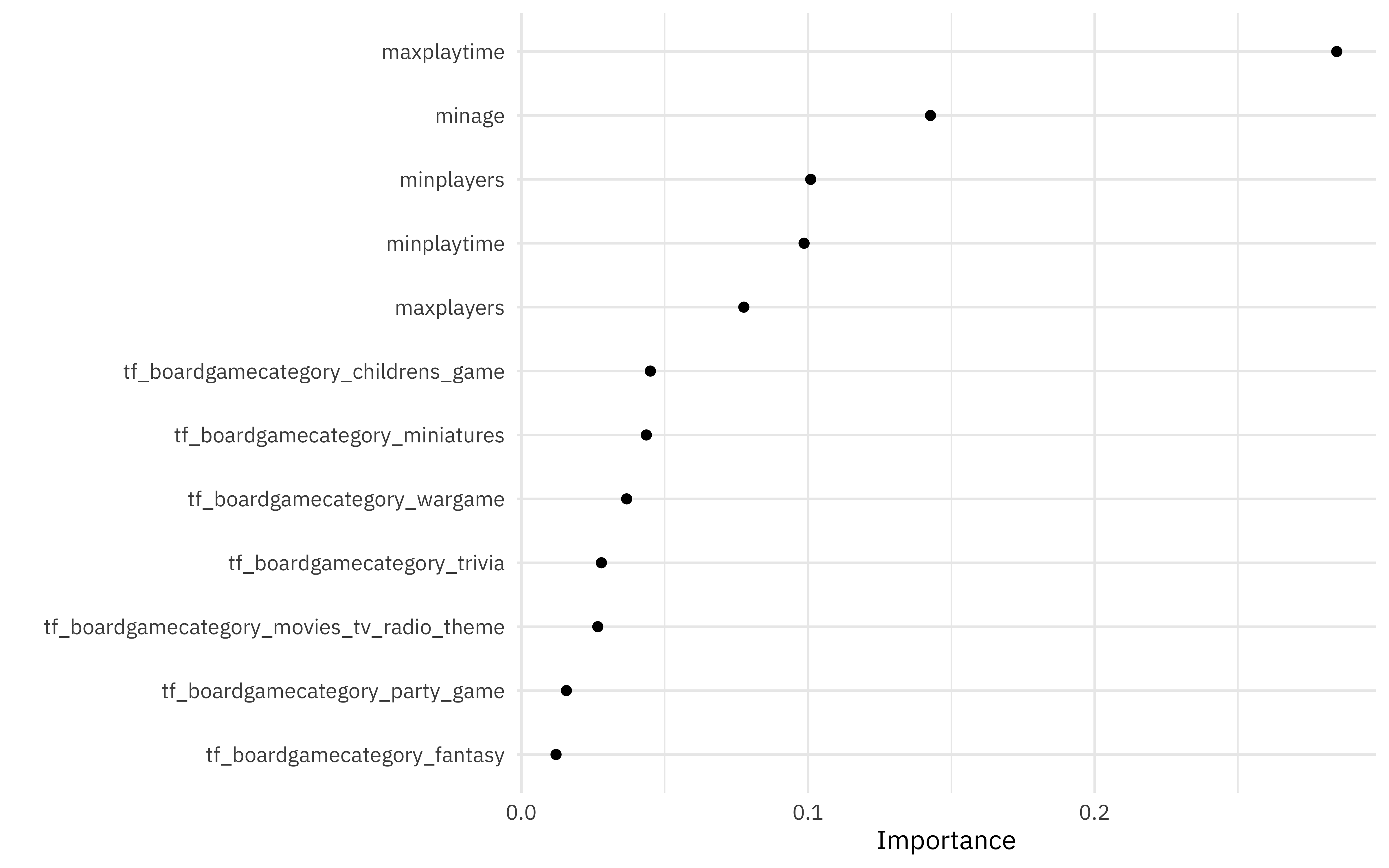
我正在尝试在 tidymodels 框架内构建一个 catboost 模型。下面给出了最小的可重现示例。我可以使用 DALEX 和 modelStudio 软件包来获取模型解释，但我想创建 VIP 绘图 像这样和总结形状图喜欢这个对于这个catboost模型。我尝试过像 fastshap、SHAPforxgboost 这样的软件包，但没有任何运气。我意识到我必须从 model 对象中提取变量重要性和形状值，并使用它们来生成这些图，但不知道该怎么做。有没有办法在 R 中完成这个工作？

library(tidymodels)
library(treesnip)
library(catboost)
library(modelStudio)
library(DALEXtra)
library(DALEX)

data <- structure(list(Age = c(74, 60, 57, 53, 72, 72, 71, 77, 50, 66), StatusofNation0developed = structure(c(2L, 2L, 2L, 2L, 2L, 
                                                                                                       1L, 2L, 1L, 1L, 2L), .Label = c("0", "1"), class = "factor"), 
               treatment = structure(c(2L, 1L, 2L, 2L, 2L, 1L, 1L, 3L, 1L, 
                                       2L), .Label = c("0", "1", "2"), class = "factor"), InHospitalMortalityMortality = c(0, 
                                                                                                                           0, 1, 1, 1, 0, 0, 1, 1, 0)), row.names = c(NA, 10L), class = "data.frame")
split <- initial_split(data, strata = InHospitalMortalityMortality)
train <- training(split)
test <- testing(split)

train$InHospitalMortalityMortality <- as.factor(train$InHospitalMortalityMortality)

rec <- recipe(InHospitalMortalityMortality ~ ., data = train)

clf <- boost_tree() %>%
  set_engine("catboost") %>%
  set_mode("classification")

wflow <- workflow() %>%
  add_recipe(rec) %>%
  add_model(clf)

model <- wflow %>% fit(data = train)

explainer <- explain_tidymodels(model,
                                data = test,
                                y = test$InHospitalMortalityMortality,
                                label = "catboost")
new_observation <- test[1:2,]
modelStudio(explainer, new_observation)

Answer 1

上面的链接提供了答案，但不完整。遵循相同的工作流程，到这里就完成了。

如图所示：首先，安装 R 软件包 {fastshap} 和 {reticulate}。接下来，使用 {reticulate} 设置一个供 python 使用的虚拟环境。使用 RStudio 时设置虚拟环境相对简单。请查看他们的参考资料以获取分步说明。

然后，在 venv 中 pip install {shap} 和 {matplotlib} - 请注意，matplotlib 3.2.2 对于摘要图似乎是必需的（有关更多详细信息，请参阅 GitHub issues）。

工作流程（来自 treesnip 文档）：

library(tidymodels)
library(treesnip)

data("diamonds", package = "ggplot2")
diamonds <- diamonds %>% sample_n(1000)

#vfolds resamples 
diamond_splits <- vfold_cv(diamonds, v = 5)

model_spec <- boost_tree(mtry = 5, trees = 500) %>% set_mode("regression")

#model specifications
lightgbm_model <- model_spec %>% 
    set_engine("lightgbm", nthread = 4)

#workflow
lightgbm_workflow <- workflow() %>% 
    add_model(lightgbm_model)

rec_ordered <- recipe( 
    price ~ .
    ,data = diamonds
)

lightgbm_fit_ordered <- fit_resamples( 
    add_recipe(
        lightgbm_workflow, rec_ordered
    ), resamples = diamond_splits
)

拟合工作流程：

fit_lightgbm_workflow <- lightgbm_workflow %>%
    add_recipe(rec_ordered) %>%
    fit(data = diamonds)

通过拟合工作流程，我们现在可以通过 {fastshap} 创建形状值，并使用 {fastshap} 和 {reticulate} 进行绘图。

首先，力图：为此，我们需要为 pred_wrapper 参数创建一个预测函数。

predict_function_gbm <- function(model, newdata){
    predict(model, newdata) %>% pull(., 1) # 
}

现在我们需要基线参数的平均预测值。

mean_preds <- mean( 
    predict_function_gbm(
      fit_lightgbm_workflow, diamonds %>% select(-price)
      ) 
)

在这里，创建形状值：

fastshap::explain( 
  fit_lightgbm_workflow, 
  X = as.data.frame(diamonds %>% select(-price)), 
  pred_wrapper = predict_function_gbm, 
  nsim= 10
) -> gbm_explained

现在，对于力图：

fastshap::force_plot( 
  object = gbm_explained[1, ],
  feature_values = as.data.frame(diamonds %>% select(-price))[1, ],
  display = "viewer", # or "html" depending on rendering preference
  baseline = mean_preds
)

# For classification, add: link = "logit"
# For vertical stacking, change: [1, ] to [1:20, ] for example. 
# this may or may not throw error depending on version of shap used.
# see {fastshap} issues.

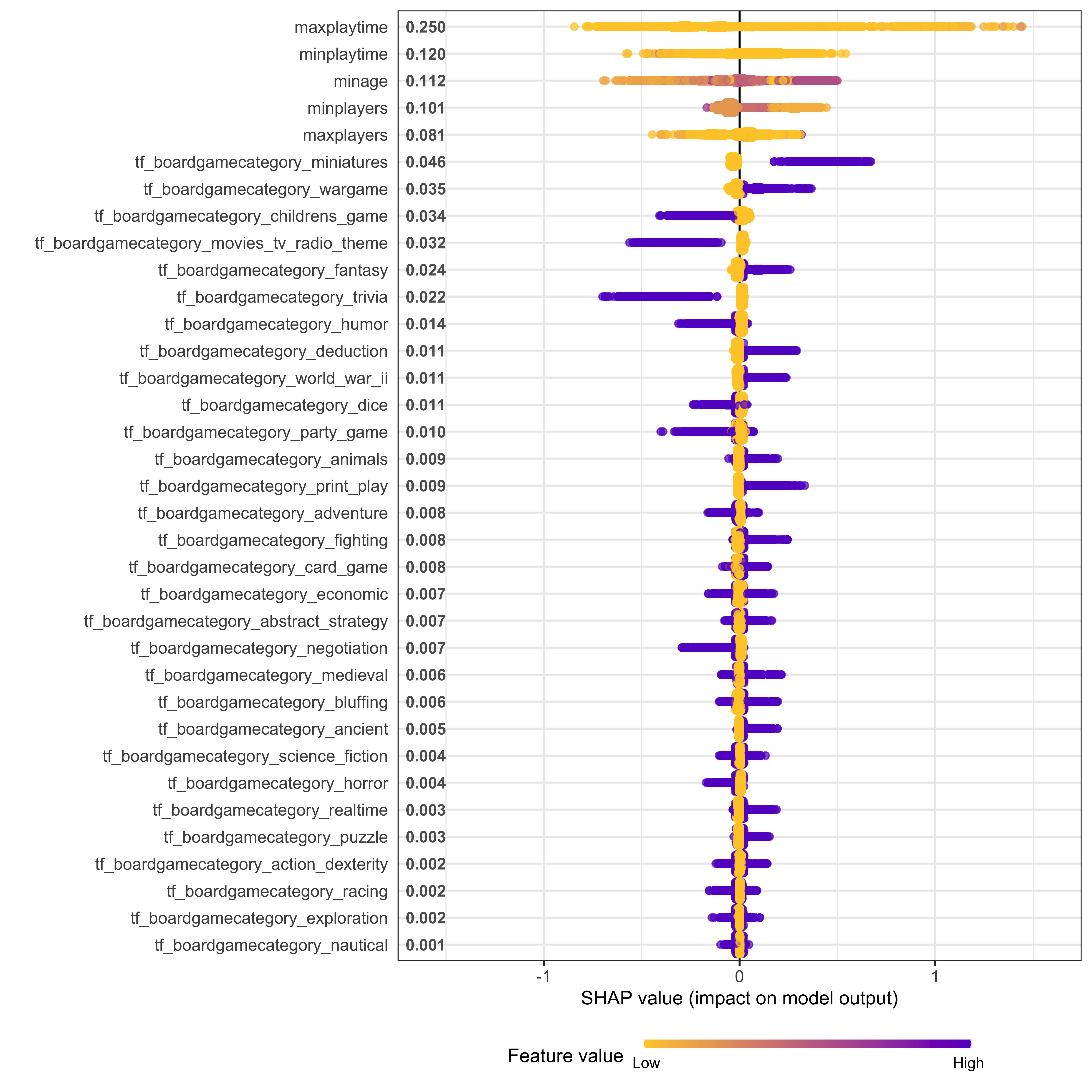
现在对于摘要图：使用 {reticulate} 直接访问函数：

library(reticulate)
shap = import("shap")
np = import("numpy")

shap$summary_plot( 
  data.matrix(gbm_explained), 
  data.matrix(diamonds %>% select(-price))
)

例如，这同样适用于依赖图。

shap$dependence_plot( 
  "rank(1)",
  data.matrix(gbm_explained), 
  data.matrix(diamonds %>% select(-price))
)

最后注意：重复渲染将导致可视化出现错误。在 dependency_plot 中直接命名一个特征（即“剪切”）给我带来了一个错误。

Answer 2

首先，我们需要从模型对象中提取工作流程，并用它来预测测试集。（可选）使用 catboost.load_pool 函数，我们创建池对象

predict(model$.workflow[[1]], test[])
pool = catboost.load_pool(dataset, label = label_values, cat_features = NULL)

之后使用 catboost.get_feature_importance 函数我们获取模型对象的特征重要性分数。

catboost.get_feature_importance(extract_fit_engine(model),
                                pool = NULL,
                                type = 'FeatureImportance',
                                thread_count = -1)

然后我们可以使用 function type = 'ShapValues' 选项获取 shapvalues。

shapvalue <- catboost.get_feature_importance(extract_fit_engine(model),
                                             pool = pool,
                                             type = 'ShapValues',
                                             thread_count = -1)
shapvalue <- data.frame(shapvalue)
shap_long_game <- shap.prep(shap_contrib = shapvalue, X_train = dataset)

最后绘制 shapvalues

shap_summplot <- shap.plot.summary(shap_long_game, scientific = F) 
shap_summplot + 
  scale_y_continuous(labels = comma)