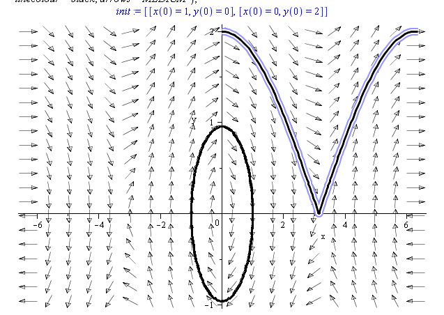
Maple ODE 求解,图形不完整。为什么?
所以我们尝试求解简单的 ODE。我们使用文本书籍(警告 - 俄语)。这是书中示例的代码(第 18 页):
> with(DEtools); with(plots);
> eq1 := diff(x(t), t) = y(t); eq2 := diff(y(t), t) = -sin(x(t));

> init := [[x(0) = 1, y(0) = 0], [x(0) = 0, y(0) = 2]];
> DEplot([eq1, eq2], [x, y], t = 0 .. 110, x = -2*Pi .. 2*Pi, init, scene = [x, y], stepsize = 0.5e-1, obsrange = true, color = black, linecolour = black, arrows = 'MEDIUM')
此代码应绘制:
但枫输出此对我来说:
1) 为什么它只解决了四分之一的功能?
2)如何解决才能使其像书上那样?
So we try to solve simple ODE. We use text book (warning - russian). This is code presented as sample in book (page 18):
> with(DEtools); with(plots);
> eq1 := diff(x(t), t) = y(t); eq2 := diff(y(t), t) = -sin(x(t));

> init := [[x(0) = 1, y(0) = 0], [x(0) = 0, y(0) = 2]];
> DEplot([eq1, eq2], [x, y], t = 0 .. 110, x = -2*Pi .. 2*Pi, init, scene = [x, y], stepsize = 0.5e-1, obsrange = true, color = black, linecolour = black, arrows = 'MEDIUM')
This code shall draw:
But maple outputs this for me:
1) Why it solves function only for one quarter?
2) How to make it solve to make it look like in the book?
如果你对这篇内容有疑问,欢迎到本站社区发帖提问 参与讨论,获取更多帮助,或者扫码二维码加入 Web 技术交流群。

绑定邮箱获取回复消息
由于您还没有绑定你的真实邮箱,如果其他用户或者作者回复了您的评论,将不能在第一时间通知您!

发布评论
评论(1)
在我看来,你所展示的情节没有任何问题。更让我惊讶的是这本书给出的情节,根据你上面粘贴的内容。想想你的初始条件。第一个是 [x(0) = 1, y(0) = 0],它从点 (1,0) 开始,并在时间上向前移动 110 个增量(根据您提供的代码)。这显然是内圈。
不过,你的第二组初始条件 [x(0) = 0, y(0) = 2] 似乎正确地从它应该的位置开始(图的顶部在点 (0,2) 处),然后它就开始了沿着场线移动,在我看来,弧长与较小的内部图大致相同。从场线来看,这更有意义。一个问题可能是在点 (pi, 0) 周围的尖点处的数字敏感问题。如果它没有在机器 epsilon 内将 y 值一路归零,那么它将到达的下一个点将爬回右上角,如图所示。
您是否尝试过使用稍微不同的初始条件和时间增量?尝试从 (-pi,0) 点开始,持续更长的时间,比如 t=0..300,看看会发生什么。有时,在这样的书中,他们选择展示的情节并不是从他们给你的代码中精确生成的,而且他们没有提到这一点。
There does not appear to me to be anything wrong with the plot you're showing. What surprises me more is the plot the book gives, according to what you've pasted above. Think about your initial conditions. The first one is [x(0) = 1, y(0) = 0], which starts at the point (1,0) and moves forward in time by 110 increments (according you your supplied code). This is clearly the interior circle.
Your second set of initial conditions though, [x(0) = 0, y(0) = 2], seems to correctly start where it should (the top of the plot at the point (0,2)) and then it does move along the field lines for what looks to me to be about the same arc length as the smaller interior plot. Judging by the field lines, this makes more sense. One issue could be numerical sensitive at the cusp around the point (pi, 0). If it doesn't get the y-value all the way to zero within machine epsilon, then the next point it will travel to will be climbing back up to the upper right as your plot shows.
Have you tried playing around with slightly different initial conditions and time increments? Try starting from the point (-pi,0) and go for much longer, say t=0..300, and see what happens. Sometimes in books like these, the plot they choose to show is not precisely generated from the code they give you and they fail to mention this.