考虑从 (-inf,inf) 到[0,1]。
(典型的 CDF 满足此属性。)
换句话说,对于任何实数 x,0 <= f(x) <= 1。
物流函数也许是最著名的例子。
现在,我们以 x 值列表的形式给出一些约束,对于每个 x 值,函数必须位于一对 y 值之间。
我们可以将其表示为 {x,ymin,ymax} 三元组的列表,例如以
constraints = {{0, 0, 0}, {1, 0.00311936, 0.00416369}, {2, 0.0847077, 0.109064},
 {3, 0.272142, 0.354692}, {4, 0.53198, 0.646113}, {5, 0.623413, 0.743102},
 {6, 0.744714, 0.905966}}
图形方式表示,如下所示:

(来源:yootles.com)
我们现在寻求一条曲线尊重这些限制。
例如:

(来源:yootles.com)
让我们首先尝试一个简单的插值通过约束的中点:
mids = ({#1, Mean[{#2,#3}]}&) @@@ constraints
f = Interpolation[mids, InterpolationOrder->0]
绘制,f看起来像这样:

(来源:yootles.com)
该函数不是满射的。此外,我们希望它更加平滑。
我们可以增加插值顺序,但现在它违反了范围为 [0,1] 的约束:

(来源:yootles.com)
那么,目标是找到满足约束条件的最平滑函数:
- 非递减。
- 当 x 接近负无穷大时趋向于 0,当 x 趋近无穷大时趋向于 1。
- 通过给定的 y 误差线列表。
我上面绘制的第一个示例似乎是一个不错的候选者,但我使用 Mathematica 的 FindFit< /a> 函数假设 对数正态 CDF。
这在这个特定示例中效果很好,但通常不需要满足约束的对数正态 CDF。
Consider the set of non-decreasing surjective (onto) functions from (-inf,inf) to [0,1].
(Typical CDFs satisfy this property.)
In other words, for any real number x, 0 <= f(x) <= 1.
The logistic function is perhaps the most well-known example.
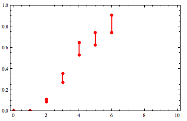
We are now given some constraints in the form of a list of x-values and for each x-value, a pair of y-values that the function must lie between.
We can represent that as a list of {x,ymin,ymax} triples such as
constraints = {{0, 0, 0}, {1, 0.00311936, 0.00416369}, {2, 0.0847077, 0.109064},
 {3, 0.272142, 0.354692}, {4, 0.53198, 0.646113}, {5, 0.623413, 0.743102},
 {6, 0.744714, 0.905966}}
Graphically that looks like this:
(source: yootles.com)
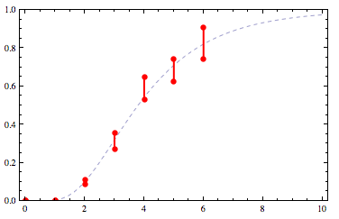
We now seek a curve that respects those constraints.
For example:
(source: yootles.com)
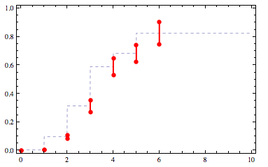
Let's first try a simple interpolation through the midpoints of the constraints:
mids = ({#1, Mean[{#2,#3}]}&) @@@ constraints
f = Interpolation[mids, InterpolationOrder->0]
Plotted, f looks like this:

(source: yootles.com)
That function is not surjective. Also, we'd like it to be smoother.
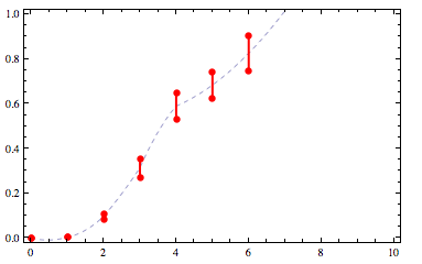
We can increase the interpolation order but now it violates the constraint that its range is [0,1]:
(source: yootles.com)
The goal, then, is to find the smoothest function that satisfies the constraints:
- Non-decreasing.
- Tends to 0 as x approaches negative infinity and tends to 1 as x approaches infinity.
- Passes through a given list of y-error-bars.
The first example I plotted above seems to be a good candidate but I did that with Mathematica's FindFit function assuming a lognormal CDF.
That works well in this specific example but in general there need not be a lognormal CDF that satisfies the constraints.


发布评论
评论(3)
我认为您没有指定足够的标准来使所需的 CDF 独一无二。
如果必须满足的唯一标准是:
那么也许你可以使用单调三次插值。
这将为您提供一个 C^2 (两次连续可微)函数,其中,
与三次样条不同,当给定单调数据时,保证是单调的。
这就留下了一个悬而未决的问题,到底应该使用什么数据来生成
单调三次插值。如果取每个误差的中心点(平均值)
吧,你能保证得到的数据点是单调的吗
增加?如果没有,你不妨做出一些任意的选择来保证
您选择的点是单调递增的(因为标准并不强制我们的解决方案是唯一的)。
现在如何处理最后一个数据点?是否有一个 X 可以保证
是否大于约束数据集中的任何 x?也许你可以再次做一个
任意选择方便,选择一些非常大的 X 并将 (X,1) 作为
最终数据点。
评论 1:您的问题可以分为 2 个子问题:
评论2:这是一种使用单调三次插值的方法,并满足条件4和5:
单调三次插值(我们称之为
f)映射R< /strong> --> R。让
CDF(x) = exp(-exp(f(x)))。然后CDF: R --> (0,1)。如果我们能找到合适的f,那么通过这种方式定义CDF,我们就可以满足条件 4 和 5。要找到
f,请变换使用转换xhat_i = x_i,yhat_i = log(-log(y_i) 的 CDF 约束。这是 CDF 变换的逆过程。如果(x_0,y_0),...,(x_n,y_n))y_i增加,则yhat_i减少。现在对 (x_hat,y_hat) 数据点应用单调三次插值以生成
f。最后,定义 CDF(x) = exp(-exp(f(x)))。这将是来自 R 的单调递增函数 --> (0,1),穿过点 (x_i,y_i)。我认为这满足了所有标准 2--5。标准 1 已得到一定程度的满足,尽管肯定存在更平滑的解决方案。
I don't think you've specified enough criteria to make the desired CDF unique.
If the only criteria that must hold is:
then perhaps you could use Monotone Cubic Interpolation.
This will give you a C^2 (twice continously differentiable) function which,
unlike cubic splines, is guaranteed to be monotone when given monotone data.
This leaves open the question, exactly what data should you use to generate the
monotone cubic interpolation. If you take the center point (mean) of each error
bar, are you guaranteed that the resulting data points are monotonically
increasing? If not, you might as well make some arbitrary choice to guarantee
that the points you select are monotonically increasing (because the criteria does not force our solution to be unique).
Now what to do about the last data point? Is there an X which is guaranteed to
be larger than any x in the constraints data set? Perhaps you can again make an
arbitrary choice of convenience and pick some very large X and put (X,1) as the
final data point.
Comment 1: Your problem can be broken into 2 sub-problems:
Comment 2: Here is a way to use monotonic cubic interpolation, and satisfy criteria 4 and 5:
The monotonic cubic interpolation (let's call it
f) maps R --> R.Let
CDF(x) = exp(-exp(f(x))). ThenCDF: R --> (0,1). If we could find the appropriatef, then by definingCDFthis way, we could satisfy criteria 4 and 5.To find
f, transform the CDF constraints(x_0,y_0),...,(x_n,y_n)using the transformationxhat_i = x_i,yhat_i = log(-log(y_i)). This is the inverse of theCDFtransformation. If they_i's were increasing, then theyhat_i's are decreasing.Now apply monotone cubic interpolation to the (x_hat,y_hat) data points to generate
f. Then finally, defineCDF(x) = exp(-exp(f(x))). This will be a monotonically increasing function from R --> (0,1), which passes through the points (x_i,y_i).This, I think, satisfies all the criteria 2--5. Criteria 1 is somewhat satisfied, though there certainly could exist smoother solutions.
我找到了一个解决方案,可以为各种输入提供合理的结果。
我首先拟合一个模型——一次拟合到约束的低端,然后再次拟合到高端。
我将这两个拟合函数的平均值称为“理想函数”。
我使用这个理想函数来推断约束结束位置的左侧和右侧,以及在约束中的任何间隙之间进行插值。
我定期计算理想函数的值,包括所有约束,从函数左侧接近零到右侧函数接近一的位置。
在约束条件下,我根据需要剪辑这些值以满足约束条件。
最后,我构建了一个遍历这些值的插值函数。
我的 Mathematica 实现如下。
首先,有几个辅助函数:
这是主要函数:
例如,我们可以拟合对数正态函数、正态函数或逻辑函数:
以下是我的原始示例约束列表的样子:
(来源:yootles.com)
正常和物流都差不多彼此重叠,对数正态是蓝色曲线。
这些都还不是很完美。
特别是,它们并不十分单调。
这是导数图:
(来源:yootles.com)
这揭示了一些缺乏平滑度的情况以及接近零的轻微非单调性。
我欢迎对此解决方案进行改进!
I have found a solution that gives reasonable results for a variety of inputs.
I start by fitting a model -- once to the low ends of the constraints, and again to the high ends.
I'll refer to the mean of these two fitted functions as the "ideal function".
I use this ideal function to extrapolate to the left and to the right of where the constraints end, as well as to interpolate between any gaps in the constraints.
I compute values for the ideal function at regular intervals, including all the constraints, from where the function is nearly zero on the left to where it's nearly one on the right.
At the constraints, I clip these values as necessary to satisfy the constraints.
Finally, I construct an interpolating function that goes through these values.
My Mathematica implementation follows.
First, a couple helper functions:
And here's the main function:
For example, we can fit to a lognormal, normal, or logistic function:
Here's what those look like for my original list of example constraints:
(source: yootles.com)
The normal and logistic are nearly on top of each other and the lognormal is the blue curve.
These are not quite perfect.
In particular, they aren't quite monotone.
Here's a plot of the derivatives:
(source: yootles.com)
That reveals some lack of smoothness as well as the slight non-monotonicity near zero.
I welcome improvements on this solution!
您可以尝试通过中点拟合贝塞尔曲线。具体来说,我认为您需要 C2 连续曲线。
You can try to fit a Bezier curve through the midpoints. Specifically I think you want a C2 continuous curve.