有条件地为 R 中置信带之外的数据点着色

发布于 2024-08-29 23:05:59 字数 1773 浏览 6 评论 0原文

我需要对下图中置信带之外的数据点与带内的数据点进行不同的着色。我是否应该在数据集中添加一个单独的列来记录数据点是否在置信区间内?您能举个例子吗?

使用置信带绘图

示例数据集:

## Dataset from http://www.apsnet.org/education/advancedplantpath/topics/RModules/doc1/04_Linear_regression.html

## Disease severity as a function of temperature

# Response variable, disease severity
diseasesev<-c(1.9,3.1,3.3,4.8,5.3,6.1,6.4,7.6,9.8,12.4)

# Predictor variable, (Centigrade)
temperature<-c(2,1,5,5,20,20,23,10,30,25)

## For convenience, the data may be formatted into a dataframe
severity <- as.data.frame(cbind(diseasesev,temperature))

## Fit a linear model for the data and summarize the output from function lm()
severity.lm <- lm(diseasesev~temperature,data=severity)

# Take a look at the data
plot(
  diseasesev~temperature,
  data=severity,
  xlab="Temperature",
  ylab="% Disease Severity",
  pch=16,
  pty="s",
  xlim=c(0,30),
  ylim=c(0,30)
)
title(main="Graph of % Disease Severity vs Temperature")
par(new=TRUE) # don't start a new plot

## Get datapoints predicted by best fit line and confidence bands
## at every 0.01 interval
xRange=data.frame(temperature=seq(min(temperature),max(temperature),0.01))
pred4plot <- predict(
                        lm(diseasesev~temperature),
                        xRange,
                        level=0.95,
                        interval="confidence"
                    )

## Plot lines derrived from best fit line and confidence band datapoints
matplot(
  xRange,
  pred4plot,
  lty=c(1,2,2),   #vector of line types and widths
  type="l",       #type of plot for each column of y
  xlim=c(0,30),
  ylim=c(0,30),
  xlab="",
  ylab=""
)

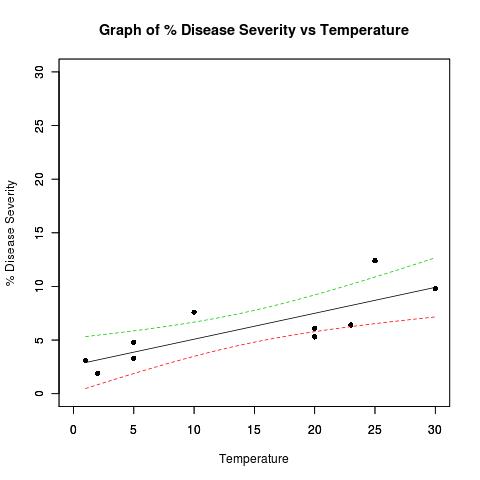
I need to colour datapoints that are outside of the the confidence bands on the plot below differently from those within the bands. Should I add a separate column to my dataset to record whether the data points are within the confidence bands? Can you provide an example please?

Plot with confidence bands

Example dataset:

## Dataset from http://www.apsnet.org/education/advancedplantpath/topics/RModules/doc1/04_Linear_regression.html

## Disease severity as a function of temperature

# Response variable, disease severity
diseasesev<-c(1.9,3.1,3.3,4.8,5.3,6.1,6.4,7.6,9.8,12.4)

# Predictor variable, (Centigrade)
temperature<-c(2,1,5,5,20,20,23,10,30,25)

## For convenience, the data may be formatted into a dataframe
severity <- as.data.frame(cbind(diseasesev,temperature))

## Fit a linear model for the data and summarize the output from function lm()
severity.lm <- lm(diseasesev~temperature,data=severity)

# Take a look at the data
plot(
  diseasesev~temperature,
  data=severity,
  xlab="Temperature",
  ylab="% Disease Severity",
  pch=16,
  pty="s",
  xlim=c(0,30),
  ylim=c(0,30)
)
title(main="Graph of % Disease Severity vs Temperature")
par(new=TRUE) # don't start a new plot

## Get datapoints predicted by best fit line and confidence bands
## at every 0.01 interval
xRange=data.frame(temperature=seq(min(temperature),max(temperature),0.01))
pred4plot <- predict(
                        lm(diseasesev~temperature),
                        xRange,
                        level=0.95,
                        interval="confidence"
                    )

## Plot lines derrived from best fit line and confidence band datapoints
matplot(
  xRange,
  pred4plot,
  lty=c(1,2,2),   #vector of line types and widths
  type="l",       #type of plot for each column of y
  xlim=c(0,30),
  ylim=c(0,30),
  xlab="",
  ylab=""
)

如果你对这篇内容有疑问,欢迎到本站社区发帖提问 参与讨论,获取更多帮助,或者扫码二维码加入 Web 技术交流群。

扫码二维码加入Web技术交流群

发布评论

需要 登录 才能够评论, 你可以免费 注册 一个本站的账号。

评论(3

倚栏听风 2024-09-05 23:05:59

好吧,我认为使用 ggplot2 这会很容易,但现在我意识到我不知道如何计算 stat_smooth/geom_smooth 的置信限。

考虑以下情况:

library(ggplot2)
pred <- as.data.frame(predict(severity.lm,level=0.95,interval="confidence"))
dat <- data.frame(diseasesev,temperature, 
    in_interval = diseasesev <=pred$upr & diseasesev >=pred$lwr ,pred)
ggplot(dat,aes(y=diseasesev,x=temperature)) +
stat_smooth(method='lm')  + geom_point(aes(colour=in_interval)) +
    geom_line(aes(y=lwr),colour=I('red')) + geom_line(aes(y=upr),colour=I('red'))

这会产生:
替代文本 http://ifellows.ucsd.edu/pmwiki/uploads/Main/strangeplot.jpg

我不明白为什么 stat_smooth 计算的置信带与直接从预测计算的带(即红线)不一致。有人能解释一下吗?

编辑:

弄清楚了。 ggplot2 使用 1.96 * 标准误差来绘制所有平滑方法的间隔。

pred <- as.data.frame(predict(severity.lm,se.fit=TRUE,
        level=0.95,interval="confidence"))
dat <- data.frame(diseasesev,temperature, 
    in_interval = diseasesev <=pred$fit.upr & diseasesev >=pred$fit.lwr ,pred)
ggplot(dat,aes(y=diseasesev,x=temperature)) +
    stat_smooth(method='lm')  + 
    geom_point(aes(colour=in_interval)) +
    geom_line(aes(y=fit.lwr),colour=I('red')) + 
    geom_line(aes(y=fit.upr),colour=I('red')) +
    geom_line(aes(y=fit.fit-1.96*se.fit),colour=I('green')) + 
    geom_line(aes(y=fit.fit+1.96*se.fit),colour=I('green'))

Well, I thought that this would be pretty easy with ggplot2, but now I realize that I have no idea how the confidence limits for stat_smooth/geom_smooth are calculated.

Consider the following:

library(ggplot2)
pred <- as.data.frame(predict(severity.lm,level=0.95,interval="confidence"))
dat <- data.frame(diseasesev,temperature, 
    in_interval = diseasesev <=pred$upr & diseasesev >=pred$lwr ,pred)
ggplot(dat,aes(y=diseasesev,x=temperature)) +
stat_smooth(method='lm')  + geom_point(aes(colour=in_interval)) +
    geom_line(aes(y=lwr),colour=I('red')) + geom_line(aes(y=upr),colour=I('red'))

This produces:
alt text http://ifellows.ucsd.edu/pmwiki/uploads/Main/strangeplot.jpg

I don't understand why the confidence band calculated by stat_smooth is inconsistent with the band calculated directly from predict (i.e. the red lines). Can anyone shed some light on this?

Edit:

figured it out. ggplot2 uses 1.96 * standard error to draw the intervals for all smoothing methods.

pred <- as.data.frame(predict(severity.lm,se.fit=TRUE,
        level=0.95,interval="confidence"))
dat <- data.frame(diseasesev,temperature, 
    in_interval = diseasesev <=pred$fit.upr & diseasesev >=pred$fit.lwr ,pred)
ggplot(dat,aes(y=diseasesev,x=temperature)) +
    stat_smooth(method='lm')  + 
    geom_point(aes(colour=in_interval)) +
    geom_line(aes(y=fit.lwr),colour=I('red')) + 
    geom_line(aes(y=fit.upr),colour=I('red')) +
    geom_line(aes(y=fit.fit-1.96*se.fit),colour=I('green')) + 
    geom_line(aes(y=fit.fit+1.96*se.fit),colour=I('green'))
我不会写诗 2024-09-05 23:05:59

最简单的方法可能是计算一个由 TRUE/FALSE 值组成的向量,该向量指示数据点是否位于置信区间内。我将稍微重新调整您的示例,以便在执行绘图命令之前完成所有计算 - 这在程序逻辑中提供了干净的分离,如果您要将其中一些打包到函数中,则可以利用该分离。

第一部分几乎相同,只是我用 severity.lm 变量替换了 predict() 中对 lm() 的额外调用- 当我们已经存储线性模型时,无需使用额外的计算资源来重新计算线性模型:

## Dataset from 
#  apsnet.org/education/advancedplantpath/topics/
#    RModules/doc1/04_Linear_regression.html

## Disease severity as a function of temperature

# Response variable, disease severity
diseasesev<-c(1.9,3.1,3.3,4.8,5.3,6.1,6.4,7.6,9.8,12.4)

# Predictor variable, (Centigrade)
temperature<-c(2,1,5,5,20,20,23,10,30,25)

## For convenience, the data may be formatted into a dataframe
severity <- as.data.frame(cbind(diseasesev,temperature))

## Fit a linear model for the data and summarize the output from function lm()
severity.lm <- lm(diseasesev~temperature,data=severity)

## Get datapoints predicted by best fit line and confidence bands
## at every 0.01 interval
xRange=data.frame(temperature=seq(min(temperature),max(temperature),0.01))
pred4plot <- predict(
  severity.lm,
  xRange,
  level=0.95,
  interval="confidence"
)

现在,我们将计算原始数据点的置信区间并运行测试以查看这些点是否在区间内:

modelConfInt <- predict(
  severity.lm,
  level = 0.95,
  interval = "confidence"
)

insideInterval <- modelConfInt[,'lwr'] < severity[['diseasesev']] &
  severity[['diseasesev']] < modelConfInt[,'upr']

然后我们将首先使用高级绘图函数 plot() 进行绘图,就像您在示例中使用的那样,但我们只会绘制区间内的点。然后,我们将使用低级函数 points() ,它将用不同的颜色绘制区间外的所有点。最后,matplot() 将用于填充您使用的置信区间。然而,我更喜欢将参数 add=TRUE 传递给高级函数,以使它们像低级函数一样运行,而不是调用 par(new=TRUE)。

使用 par(new=TRUE) 就像在绘图函数中玩弄肮脏的把戏 - 这可能会产生不可预见的后果。许多函数都提供 add 参数,使它们向绘图添加信息而不是重新绘制它 - 我建议尽可能利用此参数并依靠 par() 将操纵作为最后的手段。

# Take a look at the data- those points inside the interval
plot(
  diseasesev~temperature,
  data=severity[ insideInterval,],
  xlab="Temperature",
  ylab="% Disease Severity",
  pch=16,
  pty="s",
  xlim=c(0,30),
  ylim=c(0,30)
)
title(main="Graph of % Disease Severity vs Temperature")

# Add points outside the interval, color differently
points(
  diseasesev~temperature,
  pch = 16,
  col = 'red',
  data = severity[ !insideInterval,]
)

# Add regression line and confidence intervals
matplot(
  xRange,
  pred4plot,
  lty=c(1,2,2),   #vector of line types and widths
  type="l",       #type of plot for each column of y
  add = TRUE
)

The easiest way is probably to calculate a vector of TRUE/FALSE values that indicate if a data point is inside of the confidence interval or not. I'm going to reshuffle your example a little bit so that all of the calculations are completed before the plotting commands are executed- this provides a clean separation in the program logic that could be exploited if you were to package some of this into a function.

The first part is pretty much the same, except I replaced the additional call to lm() inside predict() with the severity.lm variable- there is no need to use additional computing resources to recalculate the linear model when we already have it stored:

## Dataset from 
#  apsnet.org/education/advancedplantpath/topics/
#    RModules/doc1/04_Linear_regression.html

## Disease severity as a function of temperature

# Response variable, disease severity
diseasesev<-c(1.9,3.1,3.3,4.8,5.3,6.1,6.4,7.6,9.8,12.4)

# Predictor variable, (Centigrade)
temperature<-c(2,1,5,5,20,20,23,10,30,25)

## For convenience, the data may be formatted into a dataframe
severity <- as.data.frame(cbind(diseasesev,temperature))

## Fit a linear model for the data and summarize the output from function lm()
severity.lm <- lm(diseasesev~temperature,data=severity)

## Get datapoints predicted by best fit line and confidence bands
## at every 0.01 interval
xRange=data.frame(temperature=seq(min(temperature),max(temperature),0.01))
pred4plot <- predict(
  severity.lm,
  xRange,
  level=0.95,
  interval="confidence"
)

Now, we'll calculate the confidence intervals for the origional data points and run a test to see if the points are inside the interval:

modelConfInt <- predict(
  severity.lm,
  level = 0.95,
  interval = "confidence"
)

insideInterval <- modelConfInt[,'lwr'] < severity[['diseasesev']] &
  severity[['diseasesev']] < modelConfInt[,'upr']

Then we'll do the plot- first a the high-level plotting function plot(), as you used it in your example, but we will only plot the points inside the interval. We will then follow up with the low-level function points() which will plot all the points outside the interval in a different color. Finally, matplot() will be used to fill in the confidence intervals as you used it. However instead of calling par(new=TRUE) I prefer to pass the argument add=TRUE to high-level functions to make them act like low level functions.

Using par(new=TRUE) is like playing a dirty trick a plotting function- which can have unforeseen consequences. The add argument is provided by many functions to cause them to add information to a plot rather than redraw it- I would recommend exploiting this argument whenever possible and fall back on par() manipulations as a last resort.

# Take a look at the data- those points inside the interval
plot(
  diseasesev~temperature,
  data=severity[ insideInterval,],
  xlab="Temperature",
  ylab="% Disease Severity",
  pch=16,
  pty="s",
  xlim=c(0,30),
  ylim=c(0,30)
)
title(main="Graph of % Disease Severity vs Temperature")

# Add points outside the interval, color differently
points(
  diseasesev~temperature,
  pch = 16,
  col = 'red',
  data = severity[ !insideInterval,]
)

# Add regression line and confidence intervals
matplot(
  xRange,
  pred4plot,
  lty=c(1,2,2),   #vector of line types and widths
  type="l",       #type of plot for each column of y
  add = TRUE
)
美胚控场 2024-09-05 23:05:59

我喜欢这个想法并尝试为此创建一个函数。当然,它还远未达到完美。欢迎您提出意见,

diseasesev<-c(1.9,3.1,3.3,4.8,5.3,6.1,6.4,7.6,9.8,12.4)
# Predictor variable, (Centigrade)
temperature<-c(2,1,5,5,20,20,23,10,30,25)

## For convenience, the data may be formatted into a dataframe
severity <- as.data.frame(cbind(diseasesev,temperature))

## Fit a linear model for the data and summarize the output from function lm()
severity.lm <- lm(diseasesev~temperature,data=severity)

# Function to plot the linear regression and overlay the confidence intervals   
ci.lines<-function(model,conf= .95 ,interval = "confidence"){
  x <- model[[12]][[2]]
  y <- model[[12]][[1]]
  xm<-mean(x)
  n<-length(x)
  ssx<- sum((x - mean(x))^2)
  s.t<- qt(1-(1-conf)/2,(n-2))
  xv<-seq(min(x),max(x),(max(x) - min(x))/100)
  yv<- coef(model)[1]+coef(model)[2]*xv

  se <- switch(interval,
        confidence = summary(model)[[6]] * sqrt(1/n+(xv-xm)^2/ssx),
        prediction = summary(model)[[6]] * sqrt(1+1/n+(xv-xm)^2/ssx)
              )
  # summary(model)[[6]] = 'sigma'

  ci<-s.t*se
  uyv<-yv+ci
  lyv<-yv-ci
  limits1 <- min(c(x,y))
  limits2 <- max(c(x,y))

  predictions <- predict(model, level = conf, interval = interval)

  insideCI <- predictions[,'lwr'] < y & y < predictions[,'upr']

  x_name <- rownames(attr(model[[11]],"factors"))[2]
  y_name <- rownames(attr(model[[11]],"factors"))[1]

  plot(x[insideCI],y[insideCI],
  pch=16,pty="s",xlim=c(limits1,limits2),ylim=c(limits1,limits2),
  xlab=x_name,
  ylab=y_name,
  main=paste("Graph of ", y_name, " vs ", x_name,sep=""))

  abline(model)

  points(x[!insideCI],y[!insideCI], pch = 16, col = 'red')

  lines(xv,uyv,lty=2,col=3)
  lines(xv,lyv,lty=2,col=3)
}

请像这样使用它:

ci.lines(severity.lm, conf= .95 , interval = "confidence")
ci.lines(severity.lm, conf= .85 , interval = "prediction")

I liked the idea and tried to make a function for that. Of course it's far from being perfect. Your comments are welcome

diseasesev<-c(1.9,3.1,3.3,4.8,5.3,6.1,6.4,7.6,9.8,12.4)
# Predictor variable, (Centigrade)
temperature<-c(2,1,5,5,20,20,23,10,30,25)

## For convenience, the data may be formatted into a dataframe
severity <- as.data.frame(cbind(diseasesev,temperature))

## Fit a linear model for the data and summarize the output from function lm()
severity.lm <- lm(diseasesev~temperature,data=severity)

# Function to plot the linear regression and overlay the confidence intervals   
ci.lines<-function(model,conf= .95 ,interval = "confidence"){
  x <- model[[12]][[2]]
  y <- model[[12]][[1]]
  xm<-mean(x)
  n<-length(x)
  ssx<- sum((x - mean(x))^2)
  s.t<- qt(1-(1-conf)/2,(n-2))
  xv<-seq(min(x),max(x),(max(x) - min(x))/100)
  yv<- coef(model)[1]+coef(model)[2]*xv

  se <- switch(interval,
        confidence = summary(model)[[6]] * sqrt(1/n+(xv-xm)^2/ssx),
        prediction = summary(model)[[6]] * sqrt(1+1/n+(xv-xm)^2/ssx)
              )
  # summary(model)[[6]] = 'sigma'

  ci<-s.t*se
  uyv<-yv+ci
  lyv<-yv-ci
  limits1 <- min(c(x,y))
  limits2 <- max(c(x,y))

  predictions <- predict(model, level = conf, interval = interval)

  insideCI <- predictions[,'lwr'] < y & y < predictions[,'upr']

  x_name <- rownames(attr(model[[11]],"factors"))[2]
  y_name <- rownames(attr(model[[11]],"factors"))[1]

  plot(x[insideCI],y[insideCI],
  pch=16,pty="s",xlim=c(limits1,limits2),ylim=c(limits1,limits2),
  xlab=x_name,
  ylab=y_name,
  main=paste("Graph of ", y_name, " vs ", x_name,sep=""))

  abline(model)

  points(x[!insideCI],y[!insideCI], pch = 16, col = 'red')

  lines(xv,uyv,lty=2,col=3)
  lines(xv,lyv,lty=2,col=3)
}

Use it like this:

ci.lines(severity.lm, conf= .95 , interval = "confidence")
ci.lines(severity.lm, conf= .85 , interval = "prediction")
~没有更多了~
我们使用 Cookies 和其他技术来定制您的体验包括您的登录状态等。通过阅读我们的 隐私政策 了解更多相关信息。 单击 接受 或继续使用网站,即表示您同意使用 Cookies 和您的相关数据。
原文