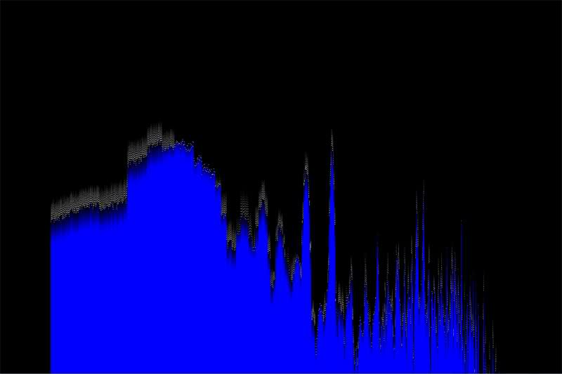
标准化 FFT 幅度以模拟 WMP

发布于 2024-08-25 17:27:39 字数 734 浏览 12 评论 0原文

所以，我一直在开发一个声音文件的小可视化工具，只是为了好玩。我基本上想模仿 Windows Media Player 中的“Scope”和“Ocean Mist”可视化工具。瞄准镜很简单，但我在使用海洋迷雾时遇到了问题。我很确定它是某种频谱，但是当我对波形数据进行 FFT 时，我没有得到与 Ocean Mist 显示的数据相对应的数据。频谱实际上看起来是正确的，所以我知道 FFT 没有任何问题。我假设可视化工具通过某种过滤器运行频谱，但我不知道它可能是什么。有什么想法吗？

编辑2：我在这里发布了代码的编辑版本（编者注：链接不再有效）。通过编辑，我的意思是我删除了所有实验性注释，只留下了活动代码。我还添加了一些描述性评论。可视化工具现在看起来像这个。

编辑：这是图像。第一个是我的可视化工具，第二个是海洋迷雾。

原文

分享到QQ

分享到微博

如果你对这篇内容有疑问，欢迎到本站社区发帖提问参与讨论，获取更多帮助，或者扫码二维码加入 Web 技术交流群。

发布评论

需要登录才能够评论，你可以免费注册一个本站的账号。

牵强ㄟ 2024-09-01 17:27:39

这是一些 Octave 代码，显示了我认为应该发生的情况。我希望语法是不言自明的：

%# First generate some test data
%# make a time domain waveform of sin + low level noise
N = 1024;
x = sin(2*pi*200.5*((0:1:(N-1))')/N) + 0.01*randn(N,1);

%# Now do the processing the way the visualizer should
%# first apply Hann window = 0.5*(1+cos)
xw = x.*hann(N, 'periodic');
%# Calculate FFT.  Octave returns double sided spectrum
Sw = fft(xw);
%# Calculate the magnitude of the first half of the spectrum
Sw = abs(Sw(1:(1+N/2))); %# abs is sqrt(real^2 + imag^2)

%# For comparison, also calculate the unwindowed spectrum
Sx = fft(x)
Sx = abs(Sx(1:(1+N/2)));

subplot(2,1,1);
plot([Sx Sw]); %# linear axes, blue is unwindowed version
subplot(2,1,2);
loglog([Sx Sw]); %# both axes logarithmic

结果如下图：
顶部：常规频谱图，底部：对数对数频谱图（蓝色为无窗）http://img710 .imageshack.us/img710/3994/spectralplots.png

我让 Octave 处理从线性到对数 x 和 y 轴的缩放。对于像正弦波这样的简单波形，您是否得到类似的结果？

旧答案

我不熟悉您提到的可视化工具，但一般来说：

光谱通常使用对数 y 轴（或光谱图的颜色图）显示。
您的 FFT 可能会返回双面频谱，但您可能只想使用前半部分（看起来您已经在这样做了）。
将窗口函数应用于时间数据可以通过减少泄漏来使频谱峰值变窄（看起来像你'我也在做这个）。
如果您关心绝对大小（我想在您的情况下并不重要），您可能需要除以变换块大小。
看起来 Ocean Mist 可视化工具也使用对数 x 轴。它还可能会平滑相邻的频率仓或其他东西。

Here's some Octave code that shows what I think should happen. I hope the syntax is self-explanatory:

%# First generate some test data
%# make a time domain waveform of sin + low level noise
N = 1024;
x = sin(2*pi*200.5*((0:1:(N-1))')/N) + 0.01*randn(N,1);

%# Now do the processing the way the visualizer should
%# first apply Hann window = 0.5*(1+cos)
xw = x.*hann(N, 'periodic');
%# Calculate FFT.  Octave returns double sided spectrum
Sw = fft(xw);
%# Calculate the magnitude of the first half of the spectrum
Sw = abs(Sw(1:(1+N/2))); %# abs is sqrt(real^2 + imag^2)

%# For comparison, also calculate the unwindowed spectrum
Sx = fft(x)
Sx = abs(Sx(1:(1+N/2)));

subplot(2,1,1);
plot([Sx Sw]); %# linear axes, blue is unwindowed version
subplot(2,1,2);
loglog([Sx Sw]); %# both axes logarithmic

which results in the following graph:
top: regular spectral plot, bottom: loglog spectral plot (blue is unwindowed) http://img710.imageshack.us/img710/3994/spectralplots.png

I'm letting Octave handle the scaling from linear to log x and y axes. Do you get something similar for a simple waveform like a sine wave?

OLD ANSWER

I'm not familiar with the visualizer you mention, but in general:

Spectra are often displayed using a log y-axis (or colormap for spectrograms).
Your FFT might be returning a double-sided spectrum, but you probably want to use only the first half (looks like you're doing already).
Applying a window function to your time data makes the spectral peaks narrower by reducing leakage (looks like you're doing this too).
You might need to divide by the transform blocksize if you're concerned with absolute magnitudes (I guess not important in your case).
It looks like the Ocean Mist visualizer is using a log x-axis too. It might also be smoothing adjacent frequency bins in sets or something.

回复收藏 0 原文